Summary
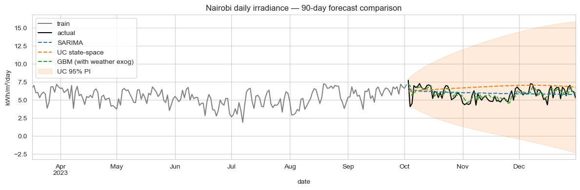
A gradient-boosted regressor that uses lagged irradiance plus same-day weather covariates (cloud cover, humidity, precipitation, temperature, wind) forecasts daily Nairobi irradiance with 9.4% MAPE across a 90-day horizon. SARIMA gets 13.8%; a UC state-space, 21.6%. Two findings worth keeping. Monthly climatology hits 12.3% MAPE (better than SARIMA), so the seasonal envelope alone explains most of the predictability. And both SARIMA and UC deliver 99% empirical PI coverage: for a battery-sizing or grid-balancing decision, the calibrated interval is what actually drives sizing, not the GBM's tighter mean.
Why this matters
Kenya runs one of the largest pay-as-you-go solar markets in Africa, with millions of household systems on sub-day battery capacity. The forecast question repeats every evening: charge the battery hard tonight, or assume tomorrow's sun will be enough? Same question at the utility level for grid integrators balancing solar against thermal and hydro. A 1-day-ahead irradiance error of 5% can flip whether a battery should be filled tonight or held in reserve. At 90-day horizons the question shifts to budgeting and storage-contract negotiation, but the metric vocabulary is the same.
The business question
Three operational consumers sit on the same forecast:
- Pay-as-you-go solar operators: battery-state-of-charge planning per household per night. Wants tight point forecasts at 1–7 day horizons.
- Utility-scale solar developers: generation expectations across 30+ day horizons; loss/over-supply decisions feed dispatch.
- Grid integrators & treasury: quantified worst-case scenarios for budgeting and risk-sharing contracts. Wants honest interval calibration.
Three customers, same forecast, three different things they look at. The case study compares a SARIMA baseline, a structural state-space model, and an ML challenger to see which fits which need.
Data
NASA POWER API: free, programmatic, no auth required. 10 years (2014-01-01 → 2023-12-31) of daily values for Nairobi (lat -1.2921, lon 36.8219):
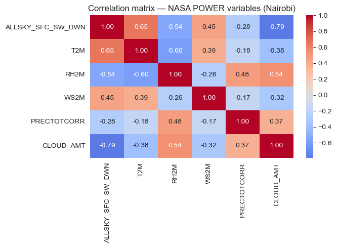
ALLSKY_SFC_SW_DWN: surface shortwave irradiance (kWh/m²/day) — the forecast targetT2M: temperature at 2 mRH2M: relative humidity at 2 mWS2M: wind speed at 2 mPRECTOTCORR: corrected precipitationCLOUD_AMT: cloud cover %
Last 90 days held out as the test window; everything before that is training. NASA POWER's free tier is generous and the API endpoint is one URL. The same pipeline switches to Lagos, Cape Town, Cairo, or Dakar by changing two numbers in download_data.py.
EDA
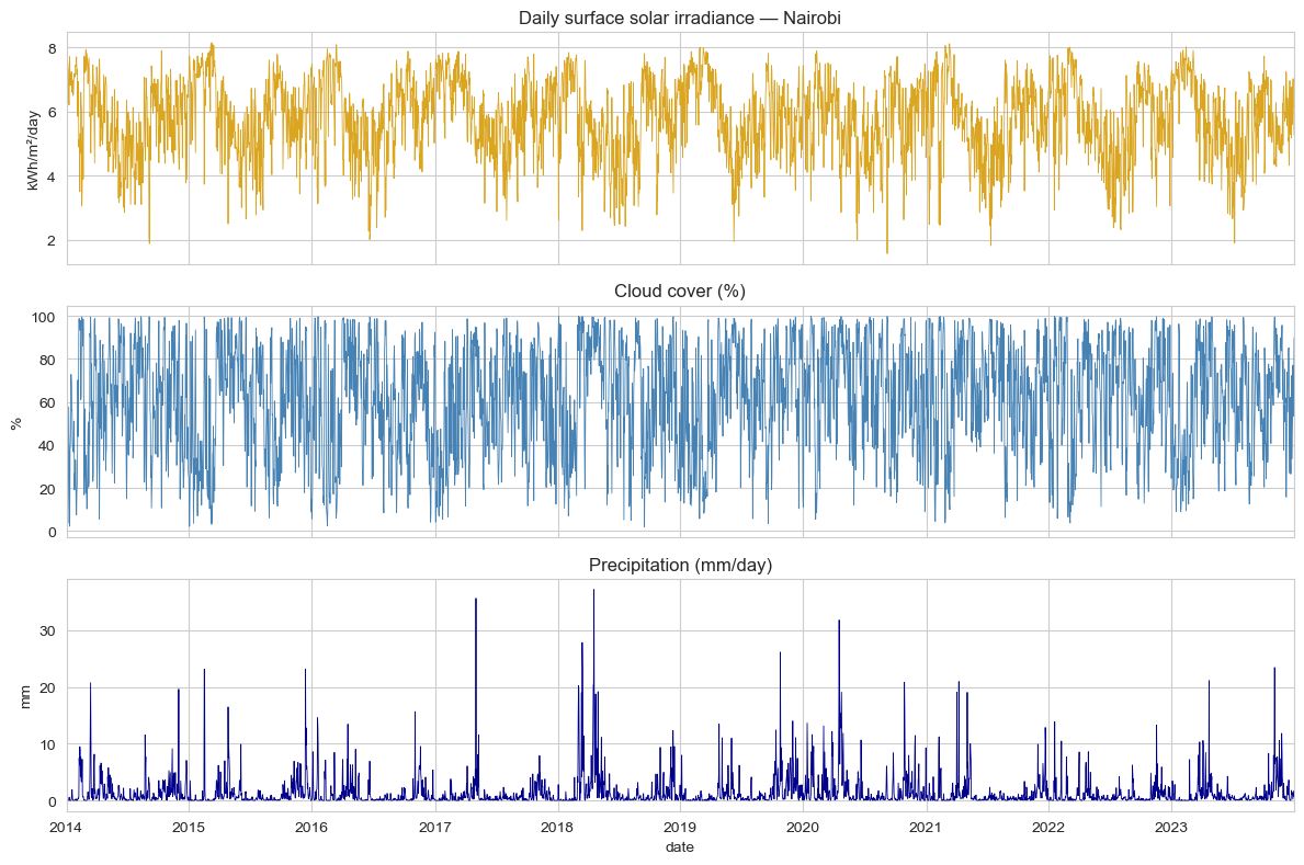
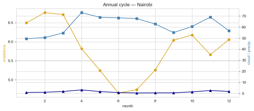
Three regularities dominate Nairobi's irradiance series, and they're physical not statistical: twice-yearly low in March–May and October–December (the "long rains" and "short rains"), twice-yearly high in January–February and July–September, and a cloud-cover anti-correlation at the daily level that's the whole story for short-horizon variance.
Modelling approach
Three primary candidates plus three baselines, all forecasting daily ALLSKY_SFC_SW_DWN 90 days ahead.
1. SARIMA
SARIMAX(2,0,2)(1,0,1)7: non-stationary AR/MA plus weekly seasonal AR/MA. Note the order. Irradiance is stationary in mean (cloud cycles oscillate around a fixed climatology), so no integration term. The weekly seasonal component is mostly absorbing measurement noise; solar isn't really a "weekly cycle" phenomenon at this latitude, but day-of-week sometimes correlates with measurement smoothing.
2. State-space — UnobservedComponents + annual Fourier exog
UnobservedComponents with local-linear-trend and four pairs of annual Fourier harmonics passed as exogenous regressors. The Fourier order of 4 is chosen because Nairobi's bimodal annual pattern needs more flexibility than a single sinusoid.
3. ML challenger — GBM with weather covariates
GradientBoostingRegressor(n_estimators=400, max_depth=3, learning_rate=0.05) on engineered features:
- Calendar:
dow,month,doy_sin,doy_cos - Lagged irradiance: 1, 2, 7, 14, 30 days
- Rolling means (shift-1): 7-day and 30-day
- Weather exogenous variables:
T2M,RH2M,WS2M,PRECTOTCORR,CLOUD_AMT: each at lag-1 and 7-day rolling mean
The cloud and humidity covariates are the lever. SARIMA and UC work only on lagged irradiance; GBM also gets yesterday's cloud cover and precipitation. The MAPE gap is mostly attributable to that information advantage.
Baselines
Three reference points: naive-last (predict tomorrow = today), naive-seasonal (predict tomorrow = irradiance one year ago), and monthly climatology (predict tomorrow = average irradiance for that calendar month, computed from the training window).
Results
90-day held-out test:
| Model | MAPE | RMSE (kWh/m²/day) | 95% PI coverage |
|---|---|---|---|
| GBM (weather exog) | 9.42% | 0.68 | — |
| Monthly climatology | 12.32% | 0.79 | — |
| SARIMA(2,0,2)(1,0,1)7 | 13.78% | 0.88 | 99% |
| Naive-seasonal (365-day lag) | 16.49% | 1.13 | — |
| UC + Fourier annual exog | 21.63% | 1.34 | 99% |
| Naive-last | 25.38% | 1.56 | — |
Trade-offs
- The GBM's gain depends on having weather data at prediction time. If the forecast is run for a date 7+ days out, you're feeding it forecast-of-forecast values for cloud/humidity, which are themselves uncertain. Production deployment needs to either (a) cap the horizon at the weather-forecast confidence horizon, or (b) chain a weather forecast model. Climatology has neither problem and is the right fallback.
- SARIMA and UC's PI coverage is the operationally useful number. 99% coverage at 95% nominal means the intervals are slightly wide; but for a battery-sizing decision, "wider but honest" is the right bias. Over-narrow intervals would be worse.
- UC underperforms on point forecast despite being structurally appropriate. The Fourier-order-4 might be overfitting to the training window's specific bimodal shape; a simpler order-2 with more noise tolerance might generalise better. Worth iterating in production.
- "Monthly climatology beats SARIMA" is a useful sanity check. It says the AR/MA structure is barely doing anything for this series. Production deployments should monitor whether SARIMA actually beats climatology on the rolling cohort — if not, ship climatology and save the compute.
Deployment sketch
For pay-as-you-go solar operators and grid integrators:
- Service: FastAPI
GET /forecast?lat=...&lon=...&horizon=30dreturning daily irradiance + 95% PI for any African coordinate. Same pipeline applies — the lat/lon parameter is the only dimension that varies. - Multi-city: NASA POWER serves the same data shape for any point on Earth; the same model artifacts work for Lagos, Cape Town, Cairo, Dakar with no code change.
- Refresh: daily cron pulls overnight NASA POWER updates; weekly retrain on the trailing 5 years; alert if rolling 30-day MAPE drifts past 12% (climatology floor).
- Dashboard: Streamlit page for solar developers showing forecast band, battery-state-of-charge simulator, and generation-impact estimator; for treasury, the same data with quantile-based scenarios.
Lessons
- Climatology is a real baseline; check it. A SARIMA that doesn't beat monthly climatology is a SARIMA that's overcomplicating the problem. The best forecast is sometimes the average of the calendar month, dressed up with a calibrated interval.
- Same-day weather covariates are the differentiator. The 4-percentage-point MAPE gain over climatology comes entirely from cloud-cover and humidity inputs. If your production system can't observe these in near-real-time, the structural model is your honest ceiling.
- NASA POWER plus a thirty-line download script is enough infrastructure for a city-level forecast service. No paid weather data, no licensing, no rate-limit anxieties. The pipeline trivially extends to any African city. The bottleneck is what you do with the forecast, not where the inputs come from.