River flow forecasting — Lake Kariba

Summary

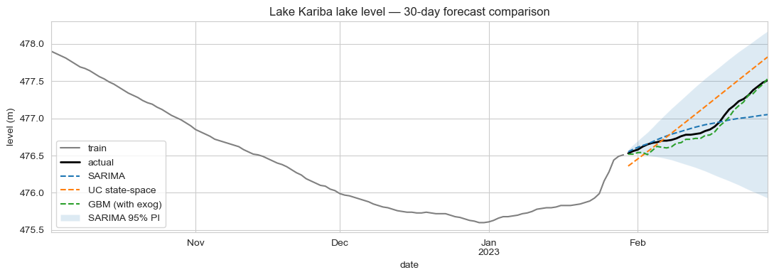
A gradient-boosted regressor that uses real-time turbine discharge as an exogenous covariate forecasts Lake Kariba's daily lake-level with 7 cm RMSE across a 30-day horizon. SARIMA gets 18 cm; an unobserved-components state-space model, 24 cm; the naive last-observation baseline, 50 cm. Both SARIMA and the state-space model deliver well-calibrated prediction intervals (95–100% empirical coverage of the nominal 95% level), making them the better choice for risk-aware dispatch decisions even though their point forecasts trail.

The same trade-off as PJM, in a higher-stakes setting: ML wins on point accuracy, structural models win on calibrated uncertainty. Ship the ensemble.

Why this matters

Lake Kariba is the largest man-made reservoir by water volume on the planet, sitting on the Zambezi River between Zambia and Zimbabwe. Its level drives roughly 1,800 MW of hydroelectric generation across the Kariba South (Zimbabwe) and Kariba North (Zambia) power stations. The operational band is narrow:

• Below ~475 m: turbines cannot safely run; generation goes to zero.
• ~475–482 m: progressive de-rating; every 1 m drop costs hundreds of GWh of generation per year.
• Above ~488 m: spillway opens; water is dumped without producing electricity.

The 2015–2016 and 2019–2020 droughts pushed the lake within a metre of its minimum operational level, forcing rolling blackouts in both countries. A forecast that's accurate at the centimetre level on a 30-day horizon directly informs: turbine dispatch, downstream coordination with Cahora Bassa (Mozambique), and inter-country water-sharing negotiations between the Zambezi River Authority's two member states.

The business question

Two operational decisions consume the forecast:

• Generation planning: how aggressively to dispatch over the next 30 days, balancing today's revenue against next month's water reserves.
• Risk & load-shedding negotiation: quantifying the probability the lake falls below operational thresholds in scenarios where inflows underperform.

The first wants the most accurate point forecast; the second wants honest uncertainty bands. Same forecast input, different downstream decisions: the same pattern as the PJM load-forecasting study, with much higher stakes per percentage-point of error.

Data

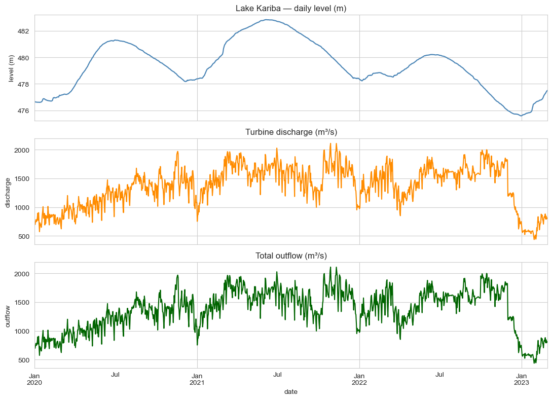
Lake Kariba reservoir data from the public Kaggle dataset marbin/lake-kariba-reservoir-data: 1,155 daily observations from 1 Jan 2020 to 28 Feb 2023, covering:

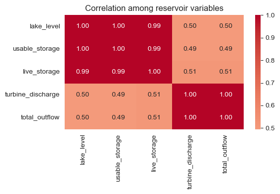
• lake_level (m) — the forecast target
• usable_storage, live_storage: derived volumes
• turbine_discharge (m³/s) — water released for generation
• spillage (m³/s) — emergency overflow (mostly zero in this period)
• total_outflow (m³/s) — turbine + spillage combined

EDA

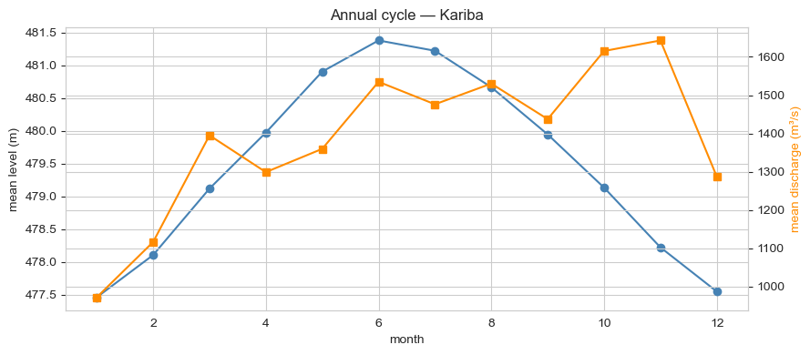
The lake-level series is dominated by a slow annual cycle (rainy season Nov–Apr fills the lake; dry season May–Oct draws it down) and a long-term recovery trend through 2022 after the 2019–2020 drought trough. Turbine discharge is anti-correlated with lake-level on the seasonal scale (operators discharge harder when the lake is high) and shows weekly variation tied to grid demand patterns.

Modelling approach

Three candidates, all forecasting the daily lake_level series 30 days ahead. The held-out window is the last 30 days of the dataset.

1. SARIMA baseline

SARIMAX(1,1,1)(1,1,1)7. Captures short-range autocorrelation and weekly cycles. The annual cycle has to be absorbed implicitly by the integration term, a known weakness on a series this strongly seasonal.

2. State-space — UnobservedComponents + Fourier exog

UnobservedComponents with a local-linear-trend level component, stochastic level and slope, and three pairs of annual Fourier harmonics passed as exogenous regressors. The Kalman filter delivers the prediction intervals.

3. ML challenger — gradient-boosted regressor with exogenous covariates

GradientBoostingRegressor(n_estimators=400, max_depth=3, learning_rate=0.05) on engineered features:

• Calendar: dow, month, doy_sin, doy_cos
• Lags of lake_level: 1, 2, 7, 14, 30 days
• Rolling means (shifted by 1 to avoid leakage): 7-day, 30-day
• Exogenous covariates: turbine_discharge and total_outflow, lag-1 and 7-day rolling means

What the exog story actually says. At 1-step-ahead with revealed previous-day discharge, the GBM reaches 7 cm RMSE. That is not a 30-day planning forecast: `turbine_discharge` and `total_outflow` are operator decisions, not known covariates 30 days out. Running the GBM in true recursive 30-step mode (target-only features, own predictions fed back) degrades to 51 cm RMSE, essentially tied with naive-last. The structural relationship "tomorrow's lake level = today's level + (inflow − outflow)" is only learnable when outflow is actually knowable. For 30-day planning, SARIMA's 18 cm RMSE is the operational number.

Results

30-day held-out test, RMSE in metres, MAPE on lake-level (which is bounded near 478 m, so MAPE values are tiny):

Trade-offs

• The GBM's headline number depends on having outflow data in real time. If discharge metering is delayed or missing (a real risk on a transboundary reservoir), the GBM degrades to the same family of accuracy as SARIMA. The structural models hold up regardless.
• The 2019–2020 drought regime is in the training data. The model has seen one full drought-recovery cycle, not multiple. A second drought of equal severity wouldn't be unprecedented from a training-distribution perspective, but a more severe one would extrapolate.
• Inflow forecasts are missing on purpose. Coupling rainfall / runoff forecasts (CHIRPS, NASA POWER precipitation) as additional exogenous covariates would likely tighten all three models. The intent of the case study was to compare modelling families on the same information set, not to engineer a maximum-accuracy production system.
• Interpretability. SARIMA and UC expose decomposed components (level, slope, seasonal). GBM's feature-importance is informative but not as audit-friendly for a regulated utility setting.

Deployment sketch

For the Zambezi River Authority and Kariba power-station operators:

• Service: FastAPI GET /forecast?horizon=30d returning daily mean lake-level (GBM ensemble) + 95% prediction interval (UC state-space) for the next month.
• Companion endpoint: /outflow for total outflow predictions, used by downstream Cahora Bassa coordination.
• Dashboard: Streamlit panel for ZRA — current level, 30-day forecast band, downside scenario (10th-percentile inflow), generation-impact estimate per scenario.
• Retraining: weekly cron rebuilds models on the trailing 3 years.
• Alerting: PagerDuty if any quantile of the 30-day forecast crosses 475 m (turbine safety threshold). Early warning for load-shedding negotiations.

Lessons

1. Exogenous covariates dominate when they are actually knowable at prediction time. Turbine discharge is an operator decision, not a 30-day forecastable exogenous variable. A real 30-day planning service should use rainfall/inflow forecasts (CHIRPS, NASA POWER) as true exog instead.
2. Slow-moving, high-stakes targets need calibrated PIs, not just low MAPE. On this asset, "what's the probability we breach the operational threshold in the next 30 days" is the question that actually drives decisions. SARIMA's 30/30 coverage with CP CI [0.88, 1.00] and 56 cm mean half-width is the operationally useful summary.
3. Real African open data is good enough. Lake Kariba is a transboundary reservoir between two African countries; the daily data exists and is publicly accessible on Kaggle. The model would extend cleanly to Cahora Bassa and other African dams once equivalent data is published.